Machine Learning 02 – Gradient Descent

Linear Regression is the most basic task of Machine Learning.

In statistics, linear regression is an approach for modeling the relationship between a scalar dependent variable y and one or more explanatory variables (or independent variables) denoted X.

We will use the following training data (they are just made up points):

features = [ 3, 2, 1, 5, 4, 7, 9 ]
targets = [ 4, 1, 4, 8, 21, 20, 26 ]

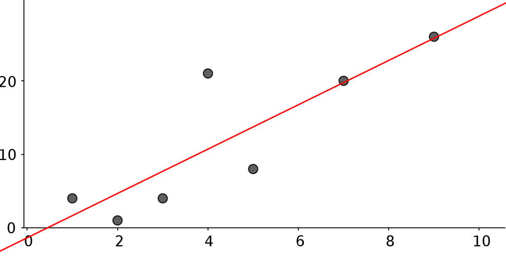
A visualization of the training data done by Geogebra. The red line shows the linear regression line ( y=3.01796 x – 1.36527 )

The solution of our problem is the function above (also called the hypothesis h(x)). To get to this solution we will use a mathematical model called least squares combined with the optimization algorithm gradient descent.

h_\theta(x) = \theta_0 + \theta_1 x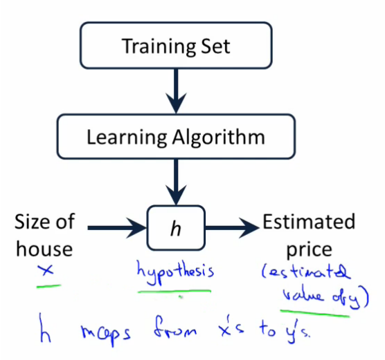

Example for training data pairs of house-size (as input) and buying-price (as output).

We are searching for the ideal $\theta_0$ and $\theta_1$ pair.

A couple of variable definitions:

m … number of training examples (in our case m = 7)
x … input Variables = features
y … output Variables = targets
(x, y) … training example
$(x^{(i)}, y^{(i)})$ … $i^{th}$ training example

We can define $\theta$ to be the vector of both $\theta_0$ and $\theta_1$ , so $\theta = \binom{\theta_0}{\theta_1}$ .

Then using the least squares method we define the function $J(\theta)=\frac{1}{2}\sum_{i=1}^{m}(h_\theta(x^{(i)})-y^{(i)})^2$ .

Using the gradient of J with respect of $\theta_i$ and updating $\theta_i$ accordingly will move us towards a local minimum.

Update rule:

\theta_i:=\theta_i-\alpha\frac{\partial}{\partial\theta_i}J(\theta)

$\alpha$ … learning rate of our learning algorithm (we will use $\alpha=0.01$ )

Choosing a good learning rate is crucial to the learning Algorithm, because a too big one can cause the $\theta_i$ to jump around, never reaching a minimum. If the learning rate is too small the algorithm will take a lot of time to reach the minimum of J ( = slow convergence).

$\frac{\partial}{\partial\theta_i}J(\theta)$ is called the partial derivative of J with respect to $\theta_i$ . We need to figure it out so we can implement it in a computer program.

\frac{\partial}{\partial\theta_i}J(\theta)=\frac{\partial}{\partial\theta_i}\frac{1}{2}\sum_{i=1}^{m}(h_\theta(x^{(i)})-y^{(i)})^2

Writing out the sum…

=\frac{\partial}{\partial\theta_i}\frac{1}{2}\Bigg[(h_\theta(x^{(1)})-y^{(1)})^2+(h_\theta(x^{(2)})-y^{(2)})^2+...+(h_\theta(x^{(m)})-y^{(m)})^2\Bigg]

We will put the factor $\frac{1}{2}$ before the derivative.

=\frac{1}{2}\frac{\partial}{\partial\theta_i}\Bigg[(h_\theta(x^{(1)})-y^{(1)})^2+(h_\theta(x^{(2)})-y^{(2)})^2+...+(h_\theta(x^{(m)})-y^{(m)})^2\Bigg]

To take the derivative of this sum, we will take the derivative of every element and sum them up.

=\frac{1}{2}\Bigg[\frac{\partial}{\partial\theta_i}(h_\theta(x^{(1)})-y^{(1)})^2+\frac{\partial}{\partial\theta_i}(h_\theta(x^{(2)})-y^{(2)})^2+...+\frac{\partial}{\partial\theta_i}(h_\theta(x^{(m)})-y^{(m)})^2\Bigg]

Here we have to use the chain rule.

=\frac{1}{2}\Bigg[2(h_\theta(x^{(1)})-y^{(1)})\frac{\partial}{\partial\theta_i}h_\theta(x^{(1)})+...+2(h_\theta(x^{(m)})-y^{(m)}))\frac{\partial}{\partial\theta_i}h_\theta(x^{(m)})\Bigg]

=(h_\theta(x^{(1)})-y^{(1)})\frac{\partial}{\partial\theta_i}h_\theta(x^{(1)})+...+(h_\theta(x^{(m)})-y^{(m)}))\frac{\partial}{\partial\theta_i}h_\theta(x^{(m)})

Now let us see what $\frac{\partial}{\partial\theta_i}h_\theta(x^{(i)})$ is…

$=\frac{\partial}{\partial\theta_i}\Big(\theta_0x^{(0)}+...+\theta_ix^{(i)}+...+\theta_nx^{(n)}\Big)$

Everything expect the $\theta_ix^{(i)}$ is just a constant, because we are deriving the function with respect to $\theta_i$ . This means that everything expect $x^{(i)}$ will be cancelled out.

Back to our derivative of J, now we can replace $\frac{\partial}{\partial\theta_i}h_\theta(x^{(i)})$ by the actual value $x^{(i)}$ .

\frac{\partial}{\partial\theta_i}J(\theta)=(h_\theta(x^{(1)})-y^{(1)})x^{(i)}+...+(h_\theta(x^{(m)})-y^{(m)}))x^{(i)}

\frac{\partial}{\partial\theta_i}J(\theta)=\sum_{j=1}^{m}(h_\theta(x^{(i)})-y^{(i)})x_i^{(j)}

So our new update rule will be:

$\theta_i:=\theta_i-\alpha\sum_{j=1}^{m}(h_\theta(x^{(i)})-y^{(i)})x_i^{(j)}$ .

We have $\theta_0$ , and $\theta_1$ , which means we will repeat updating both of them until we converge (= reach the optimal $\theta$ , that means $J(\theta)$ reaching a minimum).

I wrote a python script, to compute optimum $\theta$ vector. Note that $\theta_0$ , and $\theta_1$ became w0 and w1. The reason for choosing the letter w is that $\theta$ is sometimes also called weights.

# h(x) = O0 + O1*x1 + O2*x2 + ... + 0n*xn
# in this case: h(x) = w0 + w1*x1
features = [ 3, 2, 1, 5, 4, 7, 9 ]
targets = [ 4, 1, 4, 8, 21, 20, 26 ]
w = [ 0, 0 ] # weights w0 and w1, called Theta in Math
x = [ 1, 1 ] # x0 = 1

# alpha = 0.01
learningRate = 0.01

# actually should stop when derivative of J(w) gets near zero but we will use an iteration counter instead 
iterations = 5000 

def h(x):
    return w[0] + x*w[1]

# derivative of J = Sum j=1 to m [ h(xj) - yj ] * x1j
def derivativeJ(is_x0_soUseOneAsFactor):
    m = len(features)
    sum = 0
    for j in range(0, m):
        sum += ( h(features[j]) - targets[j] ) * ( 1 if is_x0_soUseOneAsFactor else features[j] )
    return sum

def gradientDescent():
    for j in range(0, iterations):
        w[0] = w[0] - learningRate * derivativeJ(True)
        w[1] = w[1] - learningRate * derivativeJ(False)

gradientDescent()
print( w )
# soultion for this training set h(x) = 3.01796x - 1.36527 
# correlationfactor r = 0.846