We used probability theory – and an assumption that our variables were distributed on some specific distribution like the Bernoulli or the Gaussian distribution – to construct our „hypothesis“ function and our learning algorithms.
In this Blog entry we will see that both the Bernoulli and the Gaussian distribution, even others like Poisson and Multinomial distribution all belong to a family, called the exponential family
The exponential family
For the exponential family you can define three functions b(y), T(y) and a(\eta) to get any distribution which belongs to this family. As already mentioned the Gaussian and the Bernoulli are in this family of distributions. The below formula (of the exponential family) defines a set of distributions, which are parameterized by \eta.
p(y; \eta) = b(y)*exp\big(\eta^T T(y)-a(\eta)\big)The parameter \eta is called the natural parameter. T(y) is called the sufficient statistic.
Choosing a, b and T for the Bernoulli
p(y; \phi)=\phi^y(1-\phi)^{1-y}… show that the Bernoulli distribution is just a special case of the exponential family …
b(y)=1, T(y)=y and a(\eta)=-log(1-\phi) and
\eta=log\frac{\phi}{1-\phi}thus
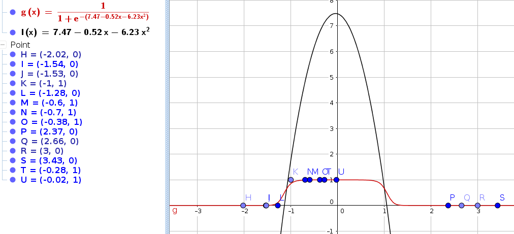
=>\phi=\frac{1}{1+e^{-\eta}}Choosing a, b and T for the Gaussian
p(y; \mu)=\frac{1}{\sqrt{2\pi}\sigma^2}exp\big(-\frac{1}{2}(y-\mu)^2\big)… show that the Bernoulli distribution is just a special case of the exponential family …
b(y)=\frac{1}{\sqrt{2\pi}\sigma^2}exp\big(-\frac{1}{2}y^2\big), T(y)=y and a(\eta)=-\frac{1}{2}\mu^2=-\frac{1}{2}\eta^2 and
\eta=\muConstruct a Generalized Linear Model (GLM)
Now that we have chosen an exponential family distribution, how do we derive a GLM? For this we will make the following three assumptions.
- y|x;\theta \sim ExpFamily(\eta) – Our first assumption states, that y is conditioned on x and parameterized by \theta are distributed by some Member of the exponential family.
- Our second assumption says that given x we want to predict an output h(x)=E[T(y)|x] which is the expected value of y. It basically says that we want to make a prediction based on the input data. The value of the prediction is the expected value of the probability distribution.
- The third assumption, we will make will set our natural parameter to be linear to our input and parameters (\eta=\theta^Tx). This assumption will be very helpful, because it allows us later to construct the Generalized Linear Model later.
construction of the GLM coming soon…