Machine Learning 04 – Locally Weighted Regression

In this blog post I will explain what the Locally Weighted Regression is and when it makes sense to use.

Picture the following data set as our given training data. We want to be able to make predictions based on the features, that’s what regression is all about.

If we use the feature $x_1=x$ our prediction function will look like this $h_\theta(x)=\theta_0 + \theta_1*x_1$ . This function is only a line. When you try to to fit a line through a data set like the one above, you will most probably get a horizontal line above the x-Axis. But its not really fitting the trends of our Data. We then could start thinking about another feature like $x_2=x_1^2$ or in this case also even $x_3=x_1x^3$ to fit our data. So the prediction function changes to: $h_\theta(x)=\theta_0+ \theta_1*x_1 + \theta_2*x^2+ \theta_3*x^3$ .

Now imagine our training data had more of a bell shape curve. We could add even more features like $x_4=sin(x)$ and so on. Another approach would be the Locally Weighted Regression (LWR) also called Loess or Lowess.

Underfitting

We talk about underfitting, when there are some patterns in the data, wich our model doesn’t recognize. For example trying to fit a straight line to more quadratic correlation.

Overfitting

Overfitting, on the other hand describes the fitting of idiosyncrasies (= a mode of behavior or a way of thought peculiar to an individual) of a specific data set. This means it’s not pattern finding more exact fitting instead of finding the underlying trends.

How to Avoid underfitting/overfitting?

To avoid underfitting/overfitting one must keep an eye on the selected features (There are algorithms to choose the best features).

„Parametric“ learning algorithm have a fixed number/set of parameters ( $\theta$ s).

„Non-Parametric“ learning algorithm: The number of parameters grow with $m$ (remember $m$ was the size of our training set).

LWR is a non-parametric learning algorithm. This algorithm will help us worry less about the features we choose.

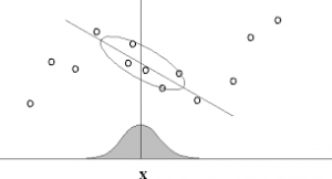
Suppose we want to make a prediction on a value $x$ . Then LWR says: Fit $\theta$ to minimize $\sum_{i=1}^m w^{(i)}(y^{(i)}-\theta^T x^{(i)})^2$ where $w^{(i)} = exp(-\frac{(x^{(i)}-x)}{2\tau^2})$ .

The differences to the „normal“ linear regression are:

The function we want to minimize looks almost the same as $J(\theta)$ , except a weight value. This weight value is calculated by a bell curved function where the peak of the bell curve is at $x$ . This means the weight gives $x^{(i)}$ s which are far away from $x$ a smaller value.
The LWR algorithm computes a new optimal $\theta$ each time we want to make a prediction. Thus, if our training set is to large this algorithm can be very costly. Although there are ways to still make it faster, these methods are not covered in the course (Stanford Machine Learning Lectures, by Andrew Ng).
It fits a line through a subset of the data, instead of trying to make a fit on the whole training data.