In this post I will explain how we can use Machine Learning to implement a binary classification algorithm.

In binary classification which is also called logistic regression our y value can only be 0 or 1. To really get a feeling for what logistic regression means I found it very helpful to look at the definition of the word logistic (of or relating to the philosophical attempt to reduce mathematics to logic). In normal regression we could have any possible y value, this time we „reduce it to logic“ so our y value can only be 0 or 1.

Because y \in {0,1} it makes a lot of sense to reduce the output of our prediction function h_\theta (x) to be in the range [0;1]. We will let h_\theta (x)   be a sigmoid function.

h_\theta (x)=g(\theta^Tx) g(z)=\frac{1}{1+e^{-z}} h_\theta (x)=\frac{1}{1+e^{-\theta^Tx}}

We will assume that P(y=1|x; \theta)=h_\theta (x). This says that the probability of y (conditioned by x and parameterized by \theta) being 1 is determined by our „hypothesis“ (=prediction function).

Thus P(y=0|x; \theta)=1 - h_\theta (x) (because y \in {0,1}).

To generalize our assumption:

P(y|x; \theta)=h_\theta (x)^y*(1 - h_\theta (x))^{1-y}

Now the question is how do we fit the parameters \theta so that the hypothesis correctly predicts the values 0 or 1 for a given x value.

To find the optimal parameters we will define a Likelihood function L which is dependent on the parameters. So we have to define L(\theta) .

L(\theta)=P(\vec{y}|X;\theta) L(\theta)=\prod_{i=1}^m P(y^{(i)}|x^{(i)};\theta) =\prod_{i=1}^m h_\theta (x)^y*(1 - h_\theta (x))^{1-y}

We will have to maximize the Likelihood of our parameters, this means we will have to maximize L(\theta). To achieve this a derivation will be needed. So we will define a logarithmic Likelihood function. We do this because it’s easier to work with logarithms, using the logarithm rules. Finding the \theta which maximized the log-Likelihood results in having found the \theta which maximizes the Likelihood function L(\theta). This is because the logarithm increases as the input of the logarithm increases.

l(\theta)=log L(\theta)=log \prod_{i=1}^m h_\theta (x)^y*(1 - h_\theta (x))^{1-y} =\sum_{i=1}^m log \Big( h_\theta (x)^y*(1 - h_\theta (x))^{1-y} \Big) =\sum_{i=1}^m log(h_\theta (x)^y) + log (1 - h_\theta (x))^{1-y} =\sum_{i=1}^m y *log(h_\theta (x)) + (1-y)*log (1 - h_\theta (x))

The update rule for our learning algorithm will look like the following:

\theta := \theta + \alpha \bigtriangledown_\theta l(\theta)

This is a gradient ascent algorithm thus we add the product of the learning rate and our derivation.

\frac{\partial}{\partial\theta_j} l(\theta)=... ... = \sum_{i=1}^m(y^{(i)}-h_\theta(x^{(i)})*x_j^{(i)} \theta_j := \theta_j + \alpha\sum_{i=1}^m(y^{(i)}-h_\theta(x^{(i)})*x_j^{(i)}

Example with a fictional Data Set

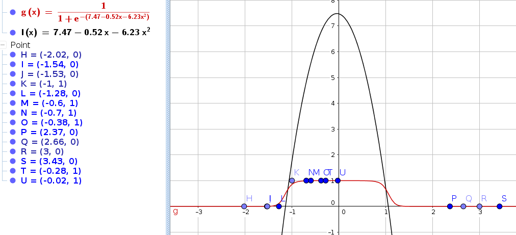
python code to classify the above points:

import math

# h(x) = g(z)
# g(z) =  1/(1+e^(-z))

points = [ 
    [-2.02, 0], 
    [-1.54, 0], 
    [-1.53, 0], 
    [-1, 1], 
    [-1.28, 0], 
    [-0.6, 1], 
    [-0.7, 1], 
    [-0.38, 1], 
    [2.37, 0], 
    [2.66, 0], 
    [3, 0], 
    [3.43, 0], 
    [-0.28, 1],
    [-0.02, 1]
]

# features
X = [ 
#   [x0=1, x1, x1^2]
    [1, points[0][0], points[0][0]**2], 
    [1, points[1][0], points[1][0]**2], 
    [1, points[2][0], points[2][0]**2], 
    [1, points[3][0], points[3][0]**2], 
    [1, points[4][0], points[4][0]**2], 
    [1, points[5][0], points[5][0]**2], 
    [1, points[6][0], points[6][0]**2],
    [1, points[7][0], points[7][0]**2],
    [1, points[8][0], points[8][0]**2],
    [1, points[9][0], points[9][0]**2],
    [1, points[10][0], points[10][0]**2],
    [1, points[11][0], points[11][0]**2],
    [1, points[12][0], points[12][0]**2],
    [1, points[13][0], points[13][0]**2]
]
# targets
y = [ 
    points[0][1],
    points[1][1], 
    points[2][1], 
    points[3][1], 
    points[4][1], 
    points[5][1], 
    points[6][1], 
    points[7][1], 
    points[8][1], 
    points[9][1], 
    points[10][1], 
    points[11][1], 
    points[12][1], 
    points[13][1]
]

w = [ 0, 0, 0 ] # weights w0 and w1, called Theta in Math

# alpha = 0.01
learningRate = 0.01
iterations = 5000 

# soultion for this training set h(x) = 3.01796x - 1.36527
# korrelation r = 0.846
def g(z): # sigmoid function
    return 1/(1+math.e**(-z))

def h(x): 
    # x = X[i] = eg.  [1, 3]
    # using sigmoid function to avoid j from getting bigger than 0 and 1 
    return g( w[0]*x[0] + w[1]*x[1] + w[2]*x[2])

# derivative of l = Sum j=1 to m [ yi - h(xi) ] * xi 
def derivativeLogLikelyHood(j): # j is number of feature, j=0 refers to x0 wich is 1, j=1 refers to x1 which is
    m = len(X) # number of trainingdata in trainingset
    sum = 0
    for i in range(0, m):
        sum += ( y[i] - h(X[i]) ) * X[i][j]
    return sum

def gradientAsscent(): # Not Descent because we want to maximize the likelikhood ..

    for iteration in range(0, iterations):
        for j in range(0, len(w)):
            w[j] = w[j] + learningRate * derivativeLogLikelyHood(j)

gradientAsscent()

print( w )